PBR论文实现：Marschner's/d'Eon Hair Model

在完成GAMES101大作业的时候，选择了Marchner的毛发模型的实现，先后参考了两篇论文，总算是做出来像个东西了。

我阅读的第一篇论文是《Light Scattering from Human Hair Fibers》，这篇文章属于是现在的毛发渲染的开山鼻祖了。

这篇论文开创性地提出了毛发的表皮含芯的模型：

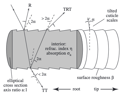
作者认为人类的毛发不是单纯的一个柱状模型（Kajiya模型），而是表皮(cuticle)加上柱芯(cortex)的组合。同时，将毛发的不同颜色归因于柱芯对于不同波长光的吸收率不同，从而导致毛发出现不同的颜色。很重要的，这个模型将光线从单纯的反射（brdf）拓展为了多个不同的类别（bcsdf），其中Marschner的这篇论文着重强调了其中的三个组成项：R、TT、RTR，R代表一次反射（reflection），T代表一次在柱芯中的传播（transmission），这里我们也可以得到，R项是没有受到吸收的，所以R项应该是造成高光的项。

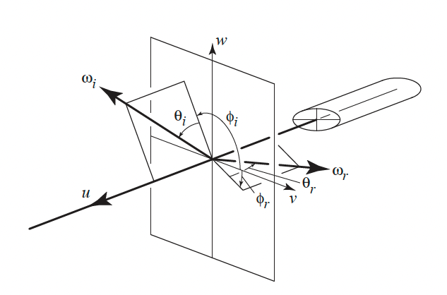
因为要直接讨论立体空间中的bcsdf会十分麻烦，因此研究者十分聪明地将一次入射投射到azimuthal和longitudinal两个方向，分别对应公式中的\(N_p\)和\(M_p\)两项，两项相乘的结果便是一个完整的入射出射得到的bcsdf。Marschner文章中的公式如下：

\[S(\phi_i, \theta_i;\phi_r,\theta_r) = M(\theta_i, \theta_r)N(\eta'(\theta_d);\phi_i,\phi_r)/\cos^2(\theta_d)\]

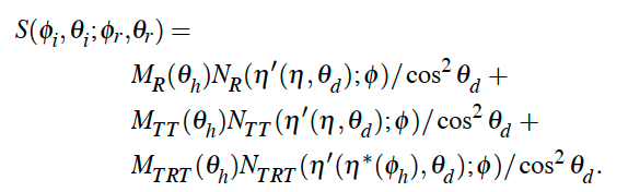
需要注意的是，因为这里有R、TT、TRT三项，对应的S也有三项，相加得到最终的答案，完整公式如下：

有了基本的思想，接下来就是对于各个子项求解了。

Longitudinal散射方程

在这个part中，我们主要和\(\theta\)项打交道，也就是我们研究和发丝径向不同夹角时产生的散射结果，有趣的是，Marschner模型的作者通过实验测量发现这个分布和高斯分布是近似的，于是我们可以通过一个标准高斯函数去逼近这个结果：

\[M_p(\theta_h)=g(\beta_p; \theta_h - \alpha_p)\]

这里的\(\beta\)和\(\alpha\)分别代表longitudinal方向的width（标准差）和shift（偏移），正好带入标准高斯方程的两个参数中。

在我阅读的第二篇论文《An Energy-Conserving Hair Reflectance Model》中，作者没有单纯的使用高斯分布，其指出使用高斯分布会导致渲染结果不遵守能量守恒（丢失大概15%），于是选用了一个符合能量守恒结果的函数：

这样得到的结果更为科学，但是在我的实现中，为了偷懒实现方便，还是选择了Marschner模型中的标准高斯分布。

对应代码：

// M term, we'll simply use gaussian distribution here
Float Mp[3];
for (int i = 0; i < 3; i++)
{
    Mp[i] = gaussian_function(beta[i], theta_h - alpha[i]);
}

Azimuthal散射方程

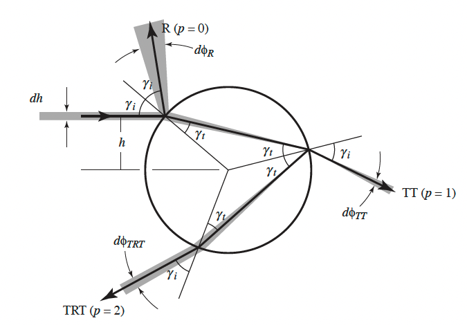
Marschner模型中对于\(N_p\)项使用了一个带微分的求和公式来准确计算散射波瓣的能量：

\[N_p(p, \phi) = \sum_rA(p, h(p,r,\phi))|2\frac{d\phi}{dh}(p, h(p,r,\phi))|^{-1}\]

根据折射反射的几何关系可以有如下的角度计算：

\[\phi(p, h) = 2p\gamma_t-2\gamma_i+p\pi\]

再加上菲涅尔项和柱芯吸收：

\[A(p,h)=(1-F(\eta',\eta'',\gamma_i))^2F(\frac{1}{\eta'}, \frac{1}{\eta''}, \gamma_t)^{p-1}T(\sigma'_a,h)^p\]

也就是说我们需要通过第二个公式求微分然后代入第一个公式，同时利用折射法则计算\(\gamma_t\)和\(\gamma_i\)的关系，很关键的，对于入射出射角，想要计算两个角度之间的关系需要利用三角函数，不利于计算，于是我们可以通过多项式拟合，再求根。但是这样要求出\(p=0,1\)的时候的解还算简单，求到\(p\ge 2\)之后，多项式的指数暴涨，要求根不太现实，不适合用于计算机求解。

于是在d'Eon11的文章里便提出了另一种方法求解\(N_p\)，那就是使用积分，通过从-1到1的h项的入射\(dh\)积分起来，模拟在出射方向的波瓣分布，来得到一个方便数值计算与预积分的解：

\[N_p(\phi) = \frac{1}{2}\int^1_{-1}A(p,h)D_p(\phi - \Phi(p,h))dh\]

同时d'Eon11这篇文章中也粗略的描述了预积分的做法：将\(\phi\)和\(\cos\theta_d\)作为两个参数构建一个二维的预计算插值表，然后运行时直接根据获取的对应的参数进行插值即可！注意，这里的积分使用的是高斯-勒让德定积分法，简单来说就是对于\(x\in[-1,1]\)的积分，选取-1到1之间的若干点，再给予各个点不同的权重，将这些点带入方程中求值之后再求和即可得到定积分的近似解。

这个公式中，使用了Gaussian Detector函数\(D_p\)来模拟出射方向上的光线分布：

\[D_p(\phi) = \sum^{\infty}_{k=-\infty}g(\beta_p;\phi-2\pi k)\]

同样的，这个函数也是可以对\(\phi\)进行预积分的：

Float gaussian_detector(Float b, Float phi) const
{
    Float result = 0;
    Float x, y, delta;
    int k = 0;
    constexpr Float M_PIx2 = M_PI * 2;
    do
    {
        x = gaussian_function(b, phi - M_PIx2 * Float(k));
        y = gaussian_function(b, phi + M_PIx2 * Float(k + 1));
        delta = x + y;
        k++;
        result += x + y;
    } while (delta > 1e-4f);
    return result;
}
for (int i = 0; i < BCSDF_TERM_NUMBER; i++)
{
    for (int j = 0; j < GAUSSIAN_DETECTOR_SAMPLES; j++)
    {
        GD_table[i][j] = gaussian_detector(beta[i], j / (GAUSSIAN_DETECTOR_SAMPLES - 1.0f) * M_PI * 2.0f);
    }
}

总体对应的预积分代码就不贴出来了，参考了Tungsten中的代码，代码链接如下：Marschner's Hair Model。

这里有一点需要注意的是，d'Eon11的文章里由于使用了新的\(M_p\)函数，所以对比的时候将原来的\(M_p\)的R项替换为了\(M_R=g(\beta_R,2\theta_h)\)来避免能量的翻倍。

最后得到的结果如下：

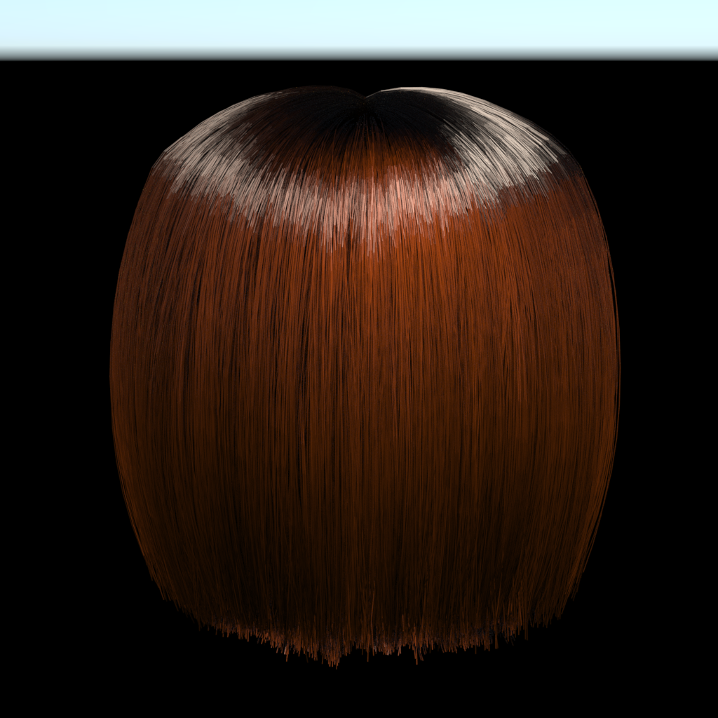
反思与思考

相比起Tungsten的渲染结果，使用我编写的bcsdf渲染得到的头发显然并不真实，很大一部分原因是因为我目前使用的重要性采样函数是一个球面的uniform采样，但是d'Eon 13文章中提出了一种新的采样策略我暂时还没有仔细研读，之后可能会考虑实现。

附录：Mitsuba的编译和配置

mitsuba的官方仓库中是这么介绍自己的：

Mitsuba is a research-oriented rendering system in the style of PBRT, from which it derives much inspiration. It is written in portable C++, implements unbiased as well as biased techniques, and contains heavy optimizations targeted towards current CPU architectures. Mitsuba is extremely modular: it consists of a small set of core libraries and over 100 different plugins that implement functionality ranging from materials and light sources to complete rendering algorithms. In comparison to other open source renderers, Mitsuba places a strong emphasis on experimental rendering techniques, such as path-based formulations of Metropolis Light Transport and volumetric modeling approaches. Thus, it may be of genuine interest to those who would like to experiment with such techniques that haven't yet found their way into mainstream renderers, and it also provides a solid foundation for research in this domain. The renderer currently runs on Linux, MacOS X and Microsoft Windows and makes use of SSE2 optimizations on x86 and x86_64 platforms. So far, its main use has been as a testbed for algorithm development in computer graphics, but there are many other interesting applications. Mitsuba comes with a command-line interface as well as a graphical frontend to interactively explore scenes. While navigating, a rough preview is shown that becomes increasingly accurate as soon as all movements are stopped. Once a viewpoint has been chosen, a wide range of rendering techniques can be used to generate images, and their parameters can be tuned from within the program.

闫令琪大大也评价Mitsuba2为最好的非商业领域渲染器，但是第一代mitsuba和第二代mitsuba的breaking change让我不得不选用第一代mitsuba来完成这篇论文的实现。

在我尝试了多个平台之后，发现最适合mitsuba1的编译安装环境还是Debian/Ubuntu等Linux操作系统上，版本不需要太过纠结。

1. 首先从Github上拉取源代码：

git clone https://github.com/mitsuba-renderer/mitsuba.git

2. 重点：切换到支持python3和scons3的分支上

git checkout scons-python3

3. 安装对应依赖

sudo apt-get install build-essential scons mercurial \
 libpng-dev libjpeg-dev \
 libilmbase-dev libxerces-c-dev libboost-all-dev \
 libopenexr-dev libglewmx-dev libxxf86vm-dev \
 libpcrecpp0v5 libeigen3-dev libfftw3-dev
pip install scons==3.0.4

4. 提取config

cp build/config-linux-gcc.py config.py

5. 在根目录下使用scons进行编译

scons -j10

这里需要说明的是，scons编译出来的版本即为开了-O3优化的版本，不需要额外指定flag。

与此同时，由于mitsuba有些年久失修，可能编译过程中会报一些奇奇怪怪的错，可以参考mitsuba仓库的issue一个一个对应修掉。

6. 设置环境变量

source setpath.sh

之后就可以在dist文件夹下面运行mitsuba来进行渲染了。